
귀퉁이 서재
DATA - 14. 통계적 유의성의 함정 본문

표본의 크기 (sample size)가 아주 크다면, 작은 차이조차도 민감하게 받아들여 어떠한 가설이라도통계적으로 유의하다는 결과가 나올 수 있습니다. 따라서 항상 대립가설을 채택하게 됩니다. 하지만 통계적으로 유의하다고, 실질적으로 유의한 것은 아니므로 주의를 해야 합니다.
With large sample sizes, hypothesis testing leads to even the smallest of findings as statistically significant. However, these findings might not be practically significant at all.
정말 표본의 크기가 크면, 통계적으로 유의한 결과가 나오는지 실습해보겠습니다. 실습용 데이터는 제 깃헙에서 받아가실 수 있습니다. (coffee_dataset.csv) 실습할 귀무가설과 대립가설은 아래와 같습니다.
귀무가설: 평균 키가 67.60이다
대립가설: 평균 키가 67.60이 아니다.
즉,
H0 : μ = 67.60
H1 : μ ≠ 67.60
표본의 크기가 5일 때
표본의 크기가 5일 때 p-value를 구해 가설검정을 해보겠습니다. 데이터 셋은 챕터 12에서 실습했었던 데이터 셋과 동일합니다.
import pandas as pd
import numpy as np
import matplotlib.pyplot as plt

%matplotlib inline
np.random.seed(42)

full_data = pd.read_csv('coffee_dataset.csv')

sample1 = full_data.sample(5)
sample1| user_id | age | drinks_coffee | height |
| 2874 | <21 | True | 64.357154 |
| 3670 | >=21 | True | 66.859636 |
| 7441 | <21 | False | 66.659561 |
| 2781 | >=21 | True | 70.166241 |
| 2875 | >=21 | True | 71.369120 |
키에 대한 모평균과 위에서 추출한 표본의 평균을 구해보겠습니다. 67.597과 67.882로 거의 유사합니다.
full_data.height.mean() # Population mean
>> 67.59748697307934
sample1.height.mean() # Sample mean
>> 67.88234252049084
이제 부트스트랩을 통해 키에 대한 표본평균 분포를 그려보겠습니다.
sampling_dist_mean5 = []

for _ in range(10000):
    sample_of_5 = full_data.sample(5)
    sample_mean = sample_of_5.height.mean()
    sampling_dist_mean5.append(sample_mean)

plt.hist(sampling_dist_mean5);
중심극한정리에 의해 거의 정규분포를 그리고 있습니다. 부트스트랩을 통해 구한 10,000개의 표본평균들의 표준편차는 1.387입니다.
std_sampling_dist = np.std(sampling_dist_mean5)
std_sampling_dist # the standard deviation of the sampling distribution
>> 1.3873129885457822
처음에 귀무가설에서 μ = 67.60이라고 가정했습니다. 따라서 null_mean = 67.60으로 변수설정을 해주겠습니다. null_vals는 평균이 null_mean이고 표준편차가 위에서 구한 1.387인 정규분포를 따르게 설정하겠습니다. 빨간 선은 맨 처음 관측한 5개의 표본의 평균입니다. 이 관측값이 null_vals로부터 나온 값인지 아닌지를 판단하는 것이 가설검정의 단계입니다.
null_mean = 67.60
null_vals = np.random.normal(null_mean, std_sampling_dist, 10000)

plt.hist(null_vals);
# where our sample mean falls on null dist
plt.axvline(x=sample1.height.mean(), color = 'red');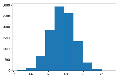
# for a two sided hypothesis, we want to look at anything
# more extreme from the null in both directions
obs_mean = sample1.height.mean()

# probability of a statistic higher than observed
prob_more_extreme_high = (null_vals > obs_mean).mean()

# probability a statistic is more extreme lower
prob_more_extreme_low = (null_mean - (obs_mean - null_mean) > null_vals).mean()

pval = prob_more_extreme_low + prob_more_extreme_high
pval
>> 0.8376
바로 이전 챕터에서 살펴본 것처럼 대립가설에 ≠ 등호가 있으면 p-value는 관측값 양 끝 영역의 합과 같습니다. 여기서는 0.8376으로 꽤 큰 값이 나왔습니다.
upper_bound = obs_mean
lower_bound = null_mean - (obs_mean - null_mean)

plt.hist(null_vals);
plt.axvline(x=lower_bound, color = 'red'); # where our sample mean falls on null dist
plt.axvline(x=upper_bound, color = 'red'); # where our sample mean falls on null dist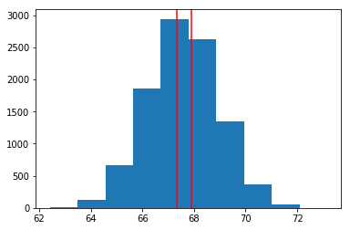
upper_bound, lower_bound
>> 67.88234252049084 67.31765747950915
빨간색 선의 오른쪽이 upper_bound, 왼쪽이 lower_bound입니다. upper_bound보다 큰 영역과 lower_bound보다 작은 영역의 합이 p-value이므로 꽤 큰 값이 맞습니다. p-value가 크기 때문에 귀무가설을 기각하지 못합니다.
표본의 크기가 300일 때
표본의 크기에 따라 가설검정의 결과가 어떻게 달라지는지 알아보기 위해, 표본의 크기가 300인 점만 빼고 모든 코드를 위와 동일하게 작성했습니다.
sampling_dist_mean300 = []

for _ in range(10000):
    sample_of_300 = full_data.sample(300)
    sample_mean = sample_of_300.height.mean()
    sampling_dist_mean300.append(sample_mean)

std_sampling_dist300 = np.std(sampling_dist_mean300)
null_vals = np.random.normal(null_mean, std_sampling_dist300, 10000)

plt.hist(null_vals);
plt.axvline(x=lower_bound, color = 'red'); # where our sample mean falls on null dist
plt.axvline(x=upper_bound, color = 'red'); # where our sample mean falls on null dist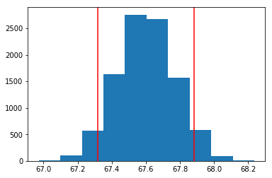
std_sampling_dist
>> 1.3873129885457822
# for a two sided hypothesis, we want to look at anything
# more extreme from the null in both directions
# probability of a statistic lower than observed
prob_more_extreme_low = (null_vals < lower_bound).mean()
# probability a statistic is more extreme higher
prob_more_extreme_high = (upper_bound < null_vals).mean()
pval = prob_more_extreme_low + prob_more_extreme_high
pval # With such a large sample size, our sample mean that is super
# close will be significant at an alpha = 0.1 level.
>> 0.09390000000000001p-value가 상당히 작아졌습니다. 유의수준이 90%라면 귀무가설을 기각해야 합니다. 똑같은 데이터인데 표본의 크기에 따라 p-value가 상당히 차이가 났고, 그에 따라 가설검정의 결과에도 서로 다른 영향을 미칠 수 있다는 점을 알게 되었습니다. 표본의 수가 커지면 작은 차이도 민감하게 반응을 해 통계적으로 유의하다는 결과가 나오는 것입니다.
본 실습을 통해 표본 크기가 상당히 클 때는 모든 가설이 통계적으로 유의할 수 있음을 알았습니다. 즉, 모든 귀무가설을 기각하는 오류가 발생할 수 있습니다. 이는 통계적으로 유의한 것이 실질적으로 유의한 것은 아니라는 것을 뜻합니다. 즉, 통계적 유의성을 너무 맹신할 필요는 없다는 뜻입니다.
'데이터 분석' 카테고리의 다른 글
| DATA - 16. A/B Test (4) | 2019.04.25 |
|---|---|
| DATA - 15. p-value의 함정 (2) | 2019.04.24 |
| DATA - 13. 가설검정과 p-value, 본페로니 교정 (6) | 2019.04.19 |
| DATA - 12. 부트스트랩(Bootstrap) (10) | 2019.04.16 |
| DATA - 11. 표본 분포, 대수의 법칙, 중심극한정리 (0) | 2019.04.14 |


