
귀퉁이 서재
컴퓨터 비전 - 8. 오토인코더 실습 본문

이전 글에서 오토인코더의 개념과 원리를 알아봤습니다. 이번 게시글에서는 오토인코더를 직접 구현해보는 실습을 다루겠습니다. 간단한 선형 인코더를 설계한 뒤, 인코딩과 디코딩을 해보겠습니다. 인코딩 결과와 디코딩 결과도 시각화해볼 겁니다.
아래 코드는 구글 코랩(colab)을 바탕으로 설명합니다.
1. 라이브러리 임포트
필요한 라이브러리를 먼저 임포트합니다.
import matplotlib.pyplot as plt
import numpy as np
import tensorflow as tf

from tensorflow.keras.models import Sequential, Model
from tensorflow.keras.layers import Dense, Input, Flatten, Reshape
from tensorflow.keras.losses import MeanSquaredError
from tensorflow.keras.datasets import fashion_mnist
2. 이미지 데이터셋 불러오기
이어서 이미지 데이터셋을 불러오겠습니다. mnist로 해도 되고, cifar-10 이미지로 해도 되지만 여기서는 fashion mnist 데이터셋을 사용해보겠습니다. fashion mnist 텐서플로에서 제공하므로 외부에서 다운로드해올 필요 없습니다. 아래와 같이 데이터셋을 불러온 뒤, 정규화까지 하겠습니다.
(X_train, y_train), (X_test, y_test) = fashion_mnist.load_data()

# Normalize
X_train = X_train / 255
X_test = X_test / 255

X_train.shape, y_train.shape
((60000, 28, 28), (60000,))
패션 mnist는 60,000개 데이터로 이루어져 있습니다. 이미지 크기는 (28, 28)이고요. 채널수가 따로 없기 때문에 흑백 이미지입니다. 테스트 데이터의 형상도 출력해보죠.
X_test.shape, y_test.shape((10000, 28, 28), (10000,))
테스트 데이터 개수는 10,000개네요. 다음으로 훈련 데이터 샘플 몇 개만 출력해보겠습니다.
plt.figure(figsize=(20, 5))

for i in range(10):
    ax = plt.subplot(1, 10, i+1)
    plt.imshow(X_train[i], cmap='gray')
    ax.get_xaxis().set_visible(False)
    ax.get_yaxis().set_visible(False)
이미지 크기가 (28, 28)이므로 해상도는 떨어집니다.
3. 오토인코더 구현한 뒤 훈련하기
이어서 오토인코더를 구현해보겠습니다. 여기서는 선형 구조로 간단하게만 설계해볼 겁니다(CNN으로 설계하면 물론 성능이 더 좋습니다).
autoencoder = Sequential()

# Encode
autoencoder.add(Flatten())
autoencoder.add(Dense(units=128, activation='relu'))
autoencoder.add(Dense(units=64, activation='relu'))
autoencoder.add(Dense(units=32, activation='relu')) # Encoded image (Latent Vector)

# Decode
autoencoder.add(Dense(units=64, activation='relu'))
autoencoder.add(Dense(units=128, activation='relu'))
autoencoder.add(Dense(units=784, activation='sigmoid'))
autoencoder.add(Reshape((28, 28)))
인코더와 디코더를 각각 설계했습니다. 먼저 인코더로 들어오는 (28, 28) 크기의 이미지를 평탄화합니다. (28, 28)를 평탄화하면 크기가 784가 됩니다. 이어서 노드 개수를 128 → 64 → 32로 줄여가면서 인코딩하게끔 했습니다. 결국 Latent Vector의 크기는 32가 됩니다. 이어서 64 → 128 →784로 늘려가면서 디코딩합니다. 마지막 계층에서 (28, 28)로 변환해 원본 이미지 크기에 맞게 만들었습니다.
다음으로 오토인코더를 빌드해야 합니다. 빌드할 때는 입력 데이터 크기를 입력해주어야 합니다.
autoencoder.build((None, 28, 28))간단한 선형 오토인코더를 만들었습니다. 전체 구조를 살펴보시죠.
autoencoder.summary()Model: "sequential_1" _________________________________________________________________
Layer (type) Output Shape Param #
=================================================================
flatten (Flatten) (None, 784) 0
dense (Dense) (None, 128) 100480
dense_1 (Dense) (None, 64) 8256
dense_2 (Dense) (None, 32) 2080
dense_3 (Dense) (None, 64) 2112
dense_4 (Dense) (None, 128) 8320
dense_5 (Dense) (None, 784) 101136
reshape (Reshape) (None, 28, 28) 0
=================================================================
Total params: 222,384
Trainable params: 222,384
Non-trainable params: 0
(28, 28) 크기의 입력 이미지를 받아서 784 크기로 평탄화하고, 128 → 64 → 32로 인코딩한 뒤, 다시 64 → 128 → 784 → (28, 28)로 디코딩하는 구조입니다.
이제 오토인코드를 훈련할 차례입니다. 훈련하기 전에 먼저 컴파일을 해야 합니다. 옵티마이저, 손실 함수, 평가지표를 다음과 같이 명시해줍니다.
autoencoder.compile(optimizer='Adam', loss=MeanSquaredError(), metrics=['accuracy'])이제 훈련을 합시다. 에폭은 50으로 설정했습니다.
autoencoder.fit(X_train, X_train, shuffle=True, epochs=50, validation_data=(X_test, X_test))4. 이미지 인코딩
훈련된 오토인코더를 활용해서 이미지를 인코딩해보고, 인코딩 결과를 시각화해보겠습니다. 먼저 인코더 모델을 만들어야 합니다. 사실 인코더 모델을 따로 만든다기보다 이미 훈련한 오토인코더에서 인코더 부분만 가져오는 겁니다. 이미지 데이터를 입력으로 받아 Latent Vector를 출력하는 레이어만 따로 떼어 모델로 만들면 됩니다. 다음과 같이 말이죠.
encoder = Model(inputs=autoencoder.input, outputs=autoencoder.get_layer('dense_2').output)여기서 inputs와 outputs에 전달한 값이 각각 무엇인지 알아보죠.
autoencoder.input<KerasTensor: shape=(None, 28, 28) dtype=float32 (created by layer 'flatten_input')>
autoencoder.input은 입력 데이터를 받는 계층입니다.
autoencoder.get_layer('dense_2').output<KerasTensor: shape=(None, 32) dtype=float32 (created by layer 'dense_2')>
autoencoder.get_layer('dense_2').output은 Latent Vector를 출력하는 계층입니다. 앞서 살펴봤던 오토인코더 구조를 보면 알 수 있습니다. 인코더를 만들었으니, 인코더 구조를 한번 살펴보죠.
encoder.summary() Model: "model"
_________________________________________________________________
Layer (type) Output Shape Param #
=================================================================
flatten_input (InputLayer) [(None, 28, 28)] 0
flatten (Flatten) (None, 784) 0
dense (Dense) (None, 128) 100480
dense_1 (Dense) (None, 64) 8256
dense_2 (Dense) (None, 32) 2080
=================================================================
Total params: 110,816
Trainable params: 110,816
Non-trainable params: 0
아래 이미지를 인코딩해보겠습니다.
plt.imshow(X_test[0], cmap='gray');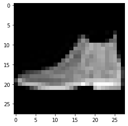
encoded_image = encoder.predict(X_test[0].reshape(-1, 28, 28))인코더에 넣을 땐 (None, 28, 28) 크기로 넣어야 해서, 형상을 변환해줜 뒤 predict() 메서드에 전달했습니다. encoder.predict()를 하면 인코딩된 Latent Vector가 encoded_image에 담깁니다. 인코딩된 이미지를 출력해보죠. (8, 4) 크기로 reshape해서 출력했습니다.
plt.imshow(encoded_image.reshape(8, 4), cmap='gray');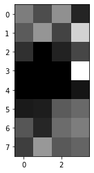
이 이미지가 신발 이미지를 인코딩한 이미지입니다. 784개(=28x28개)의 픽셀값이 단 32개(=8x4개)로 압축된 겁니다. 784개 픽셀에 담긴 중요한 정보만 가져와 32개로 압축한 거죠. 이게 Latent Vector입니다. 32개의 픽셀값, 곧 Latent Vector는 다시 디코더를 거쳐 원본 이미지와 가깝게 복원될 수 있습니다. 디코더를 만들어서 복원 작업도 해보겠습니다.
5. 이미지 디코딩
인코더와 비슷하게 디코더 모델도 만들어보겠습니다. 원리는 같습니다. 인코더는 오토인코더에서 입력부터 Latent Vector를 만드는 계층까지를 추출했다면, 디코더는 Latent Vector를 만드는 계층 바로 다음 계층부터 마지막 계층까지 추출해서 만들면 됩니다.
input_layer_decoder = Input(shape=(32,))
decoder_layer1 = autoencoder.get_layer('dense_3')
decoder_layer2 = autoencoder.get_layer('dense_4')
decoder_layer3 = autoencoder.get_layer('dense_5')
decoder_layer4 = autoencoder.get_layer('reshape')
decoder = Model(inputs=input_layer_decoder, outputs=decoder_layer4(decoder_layer3(decoder_layer2(decoder_layer1(input_layer_decoder)))))
이렇게 만든 디코더에 Latent Vector를 전달해 디코딩해보겠습니다.
decoded_image = decoder.predict(encoded_image)잘 디코딩이 되었는지, 즉 잘 원복됐는지 시각화해볼까요?
plt.imshow(decoded_image.reshape(28, 28), cmap='gray');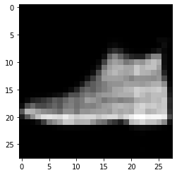
상당히 잘 복원이 되었습니다. 아래가 원본 이미지인데, 원본 이미지와 크게 차이가 없네요.

6. 원본 이미지 - 인코딩 이미지 - 디코딩 이미지 시각화
열 가지 샘플 이미지를 활용해 인코딩, 디코딩 이미지를 시각화해보겠습니다. 원본 이미지와 원복 이미지(디코딩 이미지)를 비교해보세요. 디코딩된 원복 이미지가 원본 이미지와 같을수록 오토인코더의 성능이 좋은 겁니다.
num_of_images = 10

plt.figure(figsize=(20, 7))
for i in range(num_of_images):
    # Origianl images
    ax = plt.subplot(3, 10, i+1)
    plt.imshow(X_test[i], cmap='gray')
    plt.title("Original")
    ax.get_xaxis().set_visible(False)
    ax.get_yaxis().set_visible(False)

    # Encoded images
    ax = plt.subplot(3, 10, i+1+num_of_images)
    encoded_image = encoder.predict(X_test[i].reshape(-1, 28, 28))
    plt.imshow(encoded_image.reshape(8, 4), cmap='gray')
    plt.title("Encoded")
    ax.get_xaxis().set_visible(False)
    ax.get_yaxis().set_visible(False)

    # Decoded images
    ax = plt.subplot(3, 10, i+1+2*num_of_images)
    decoded_image = decoder.predict(encoded_image)
    plt.imshow(decoded_image.reshape(28, 28), cmap='gray')
    plt.title("Reconstructed")
    ax.get_xaxis().set_visible(False)
    ax.get_yaxis().set_visible(False)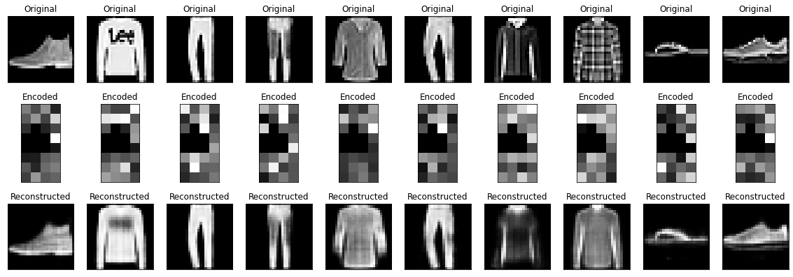
모양은 대체로 비슷하게 원복을 했습니다. 그런데, 티셔츠의 프린팅이나 체크무늬 셔츠의 체크 패턴은 원복을 못했습니다. 아무래도 선형 오토인코더라서 성능이 썩 좋진 않네요. CNN으로 구현하면 성능이 더 좋아질 겁니다.
참고 자료
'컴퓨터 비전' 카테고리의 다른 글
| 컴퓨터 비전 - 10. R-CNN vs. SPP-net vs. Fast R-CNN vs. Faster R-CNN 개요 (4) | 2023.03.15 |
|---|---|
| 컴퓨터 비전 - 9. 객체 탐지(Object Detection) 개요 (4) | 2023.03.14 |
| 컴퓨터 비전 - 7. 오토인코더(AutoEncoder)와 매니폴드 학습(Manifold Learning) (4) | 2023.03.12 |
| 컴퓨터 비전 - 6. 영상에서 감정 분류하기 (2) | 2023.03.10 |
| 컴퓨터 비전 - 5. 얼굴 이미지에서 감정 분류(Emotion Classification) (0) | 2023.03.09 |


